Built-in Self -Test - Laboratory work 3

Topic: Built-in Self-Test - Laboratory work 3

1. Test Generation
2. Design Error Diagnosis
3. Built-in Self-Test

3.1. Example

4. Design for Testability

3. BUILT-IN SELF-TEST

Objectives
To explore and to compare different built-in self-test techniques. To learn finding best LFSR architectures and initial states (seeds) for BILBO and CSTP methods. To learn finding best combinations of stored and generated patterns in the Hybrid BIST approach.

Introduction
It is often needed to test an already installed and working device to be sure that it operates properly. It is not convenient and often not even possible to take the device off its working place to test it with the external ATE (automated test equipment). Various embedded test techniques are used in such cases. This approach is commonly called the built-in self-test (BIST). It usually implies the presence of one or more built-in linear feedback shift registers (LFSR) to generate test patterns and analyze acquired signatures. The BILBO (Built-In Logic Block Observer) method, for example, needs two LFSRs. One for test generation, another for signature analysis. In the CSTP (Circular Self-Test Path) just a single LFSR is used for the both purposes.

However, the major drawback of LFSR-based methods is that the test can be too long to be performed within a given period of time. This is due to the properties of test sequences generated by the LFSR. There is a number of so called Hybrid BIST methods designed to fight the problem of too long sequences. One of them, "store & generate" implies the use of some stored seeds for the LFSR. From these seeds a set of smaller sequences is generated. The total length of them is much less than the length of the single test sequence generated by the BILBO or CSTP.

Work description
Suppose, we have a system on a chip with a number of functional units. Three of them are combinational circuits, which must be tested by a single BIST device to save the silicon area and hardware costs. To do so, we are going to use the "broadcasting BIST" technique which is illustrated in the following picture.

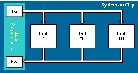
This technique implies that the test generator (TG) sends simultaneously the same vectors to all the units under test. The output responses (all together) are analyzed in the response analyzer (RA). The particular implementation of TG and RA may depend on the BIST architecture (like BILBO or CSTP). Our task is to choose the architecture and the initial state of the LFSR in TG so that it would generate a good test sequence for all the three circuits simultaneously. One of the possible approaches to solve this problem is the following.

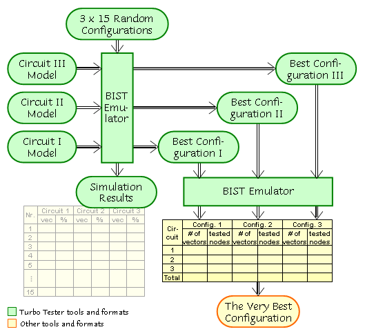
First, we select a good configuration (architecture-seed pair) for each circuit separately. For that we use 3 times 15 random configurations, simulate them, and register the simulation results. Using these results we choose the three best configurations. Then we simulate all of them one after another with each of the three circuits and register results again. Finally we must choose the best configuration - an architecture-seed pair that gives the highest total fault coverage or/and the shortest test length. During our work we will examine both BILBO and CSTP methods and then compare their efficiency.

Another problem to be solved during this work is to find an optimal (or suitable) to given constraints combination of stored seeds and generated test patterns for "store & generate" - one of the techniques in Hybrid BIST approach. Suppose we have another chip with a circuit that has to be periodically tested. At the same time, we have a strictly limited testing time and therefore cannot use a conventional LFSR for test generation. There is also a limitation of a chip space. In these harsh conditions we have to find the solution anyway. So, our task can be bilateral: a) to find a minimum number of good seeds when the upper test length limit L is known or b) to find such seeds that give the shortest total test length if the maximim number of seeds S is given. The task can be even tougher if we are requested to minimize the both parameters.

Steps

Choose the proper length of the TPG (Test Pattern Generator) and SA (Signature Analyser) for the case of BILBO. The length must be consistent to the number of inputs and outputs of all the three given circuits.
Take the circuits one by one and for each one try to find the seed that gives a possibly better fault coverage or/and test length. Use BIST emulator in BILBO mode for that purpose. Change architectures (LFSR polynomial) of the TPG and the SA and choose different seeds to improve fault coverage. Try at least 15 different configurations for each circuit. You have to obtain three best BILBO configurations (one for each circuit) at the end of the phase.
Take the first configuration and apply it to the second and the third circuit. Take the second configuration and apply it to the first and the third circuit. Take the third one and apply it to the first and the second circuits. Choose the configuration that gives the best total coverage with the minimal total test length.
Repeat steps 1-3 for CSTP. However, note that the TPG and the SA parts are united in one LFSR. Use BIST emulator in CSTP mode. Compare the efficiency of CSTP and BILBO methods.
Write the schedule for the Hybrid BIST device. For that purpose select the first circuit among the three and select the best BILBO confuguration that you have got during step 2. The test sequence length of this configuration will be the initial vector count L. The target vector count is L/2. Your main task is to find the minimal number S of stored seeds to approach the target test length.
Compare the efficiency of all the investigated BIST techniques. Which method is better: Hybrid BIST or BILBO if each stored seed costs us as much as 50 generated test vectors?

3.1 Example

Steps

The circuits that we use in the exapmle are given in Table 1 below. The maximal numbers of inputs and outputs among all of them are 36 and 25 respectively. This means that the minimal length of the TPG must be 36 bit and the minimal length of the SA is 25 bit. For CSTP, the LFSR's minimal length must be taken as 36 bit.

TABLE 1
Circuit Name	Number of Inputs	Number of Outputs	File Name
c17	5	2	c17.agm
c432	36	7	c432.agm
c1908	33	25	c1908.agm

To generate a pseudo random sequence by the BIST emulator in BILBO mode write: bist -rand -glen 36 -alen 25 -optimize -simul bilbo c17. We have made a lot of experiments with different random (-rand option) configurations for c17 circuit and registered the results, which (15 of them as it is required) we give in Table 2 . The simulation has shown that it is always possible to achieve 100% coverage with any chosen BILBO architecture and random seed for our circuit. What changes from experiment to experiment is the test length. The best one is 7 vectors only (highlighted in green). The corresponding configuration (architecture/seeds), the nr. 6 configuration is chosen as the best for this circuit (since the coverage has always been the same). It is given in Table 3.

TABLE 2
	Circuit 1		Circuit 2		Circuit 3
Nr.	# of vectors	Fault cover. %	# of vectors	Fault cover. %	# of vectors	Fault cover. %
1	11	100.00	435	93.019	5582	99.480
2	19	100.00	427	93.019	5711	99.480
3	21	100.00	589	93.019	8875	99.480
4	25	100.00	314	93.019	9842	99.307
5	19	100.00	1459	93.019	6119	99.480
6	7	100.00	363	93.019	5075	99.480
7	12	100.00	1473	93.019	8876	99.480
8	20	100.00	1675	92.857	9818	99.480
9	19	100.00	982	93.019	4034	99.480
10	45	100.00	1671	93.019	7415	99.480
11	14	100.00	300	91.396	5671	98.210
12	37	100.00	767	93.019	8771	99.365
13	21	100.00	656	93.019	5718	99.480
14	10	100.00	1405	93.019	6781	99.480
15	18	100.00	867	93.019	4761	99.480

We continued then the experiments with the two remaining circuits in the similar way. In the case of c432 circuit, the best vector count was 300. However, at the same time the fault coverage was lower than in other cases. Therefore, we selected the best test length among the results with the best fault coverage. It was the case nr. 4. Again, we put it in Table 3. The experiments with c1908 has shown that the corresponding configuration nr. 9 is the best. For each of the given circuits we selected -count option for the BIST emulator based on recommendation given here. For c432 we used -count 1500, while for c1908 -count 10000. When we use -count and -optimize options together we force the emulator to generate the specified number of vectors or stop at some point if the coverage does not improve any further. When you will be performing your experiments do not forget to copy the file withe the best so far BIST configuration to another file with an arbitrary name (e.g. cp c432.tst c432.best)! Otherwise, it will be each time overwritten!

TABLE 3
Circuit Name	Number of Vectors	Fault Coverage, %	TPG seed TPG Architecture SA Seed SA Architecture
c17	7	100.00	110000100110101001111111011010011110 101011011100100111001011110001011001 0010010001001010010010010 1101000010010010110001110
c432	314	93.019478	110000100110101001100001001101111110 101011011100100101000100010011011001 0010010001001010001110001 1101000010010010101110010
c1908	4034	99.480370	110000100110101001110111110000011110 101011011100100101100110001010111001 0010010001001010100000111 1101000010010010111010101

As it was stated above, each time we were taking a new random BIST configuration and simulated it. However, there is another good strategy to acquire "good" BIST configurations. Propably, you will notice from your experiments that "good" polynomials are always very similar. So, this means that it should be possible to generate new better polynomials by introducing minor changes into initial ones. You can try this method as well. Likely, it will give you better results within shorter time!

So far, we have three good BIST configurations. All of them are good for the corresponding circuit and we need to find out which one is the best for all the circuits taken together. To make a prediction, we can say that the best configuration should be probably that one, which is the best for the largest circuit. In our case it is that one, which gives 4034 vectors for c1908. It is very likely, that any other configuration applied to this circuit will result in a longer test. Which means the longer total test length since we use the Broadcasting BIST approach, when all the circuits are tested simultaneously.

To apply the first configuration to c432 circuit write: bist -ginit 110000100110101001111111011010011110 -gpoly 101011011100100111001011110001011001 -ainit 0010010001001010010010010 -apoly 1101000010010010110001110 -optimize -simul bilbo -count 10000 c432. All other configurations are applied to all the circuits in the similar way.

The results of the simulation are given in Table 4 below. It shows the test lengthes and fault coverage for each BIST configuration and each circuit. The best length for each particular circuit is highlighted, again, by green. The fault coverage is given now as the number of tested nodes (not the percentage). This is useful for calculation of the total coverage, which is given in the last row of the Table 4. This row also shows the maximal test length for each configuration. The best one is highlighted by green.

TABLE 4
Config:	Configuration 1		Configuration 2		Configuration 3
Circuit	# of vectors	Tested nodes	# of vectors	Tested nodes	# of vectors	Tested nodes
c17	11	22	19	22	19	22
c432	589	573	314	573	1459	573
c1908	7415	1723	8875	1723	4034	1723
Max/Total:	7415	2318	8875	2318	4034	2318

The experiments with CSTP approach are very similar to those we made for BILBO. To run BIST emulator in CSTP mode, use -simul cstp option. For instance: bist -rand -glen 36 -optimize -simul cstp c17. Since the CSTP unit has a single LFSR register for both the generator and analyzer, the length of such a register should be greater or equal to the greatest number of inputs or outputs among all the circuits under test (see Step 1). Use here -glen, -ginit, or/and -gpoly options only. No -alen, -ainit, or -apoly necessary for CSTP!
For Hybrid BIST scheduling use the report tool together with -progress option. Find the ranges in the test sequence when the fault coverage does not increase. Remove as much of these ranges as needed to reduce the initial sequence length by the factor of 2. After each such removal the first vector after the last removed must be stored in the memory as the next seed. Remember, that your task is to solve the problem using the minimal number of such seeds!
Compare the efficiency of the investigated BIST techniques. Take the test length and the fault coverage as the measure here. Which BIST configuration is the best for the investigated set of circuits? Which BIST mode (BILBO or CSTP) is better in your case? Which method is better: Hybrid BIST or BILBO if each stored seed costs us as much as 50 generated test vectors?

Last update: 23 October, 2002 by Artur Jutman